Building a GPU Compiler from Scratch
Lowering PyTorch Graphs to CUDA via Multi-Level IRs
In 2018, a friend and I started building the lowering stack for the Apple Neural Engine. We had little idea how to build an ML compiler; neither of us had built much of any compiler before. To my surprise, building it today, eight years later, still feels like pioneering. The field is a boiling pot of frameworks, ideas, techniques, and plain hacks. We keep adding ingredients, but still argue over the recipe.
I’ll attempt the soup base. The IR stack and progressive lowering are about as close to settled ideas as this field gets.
In this tutorial, we will follow one PyTorch operation down to CUDA via progressive lowering, and see why each compiler stage exists through small, reproducible examples.
To follow along, create a Python 3.12 or newer virtual environment and install Emmy 0.3.22. You can inspect the IR without a GPU; running the benchmarks later requires an NVIDIA GPU and nvcc.
python3 -m venv emmy_venv
source emmy_venv/bin/activate
python -m pip install "emmy-ml[compile]==0.3.22" "torch==2.14.1"
export EMMY_TUNE_DB="$(mktemp -d)/tutorial.db"
export EMMY_GOLDEN_FILE=
Pipeline
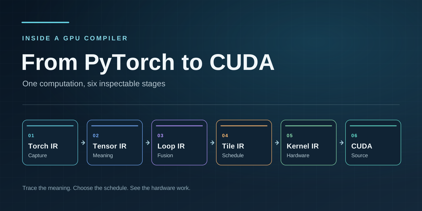
An IR, or intermediate representation, describes a program at one stage of compilation. Take an FP16 matmul C = A @ B, where A is [M,K] and B is [K,N]. The sketches show how the same computation gains detail at all six stages:
| Stage | What it adds | Simplified matmul example |
|---|---|---|
| Torch IR | Captures the framework operation | C = matmul(A, B) |
| Tensor IR | Makes indexing and reduction explicit | A_bc[i,k,j] = A[i,k]B_bc[i,k,j] = B[k,j]C[i,j] = sum_k(A_bc[i,k,j] * B_bc[i,k,j]) |
| Loop IR | Fuses the scalar loops | for i in 0..M: for j in 0..N: acc = 0 for k in 0..K: acc += A[i,k] * B[k,j] C[i,j] = acc |
| Tile IR | Separates computation from its schedule | C[i,j]: Fold[k] (lift a*b, combine +) ├─ load A[i,k] └─ load B[k,j] |
| Kernel IR | Spells out hardware work | LoadTile(A, shared)LoadTile(B, shared)SyncMMA(acc, A_frag, B_frag)Store(C_tile) |
| CUDA | Emits source for nvcc | global void matmul(...) { int i = blockIdx.y; int j = blockIdx.x * blockDim.x + threadIdx.x; if (j >= N) return; float acc = 0; for (int k = 0; k < K; ++k) { acc += float(A[iK+k]) * float(B[kN+j]); } C[i*N+j] = acc;} |
Throughout the article, we'll use RMSNorm as an example. For a row of length and learned weight , each output element is:
First, it computes the mean of the squared row elements, adds , and takes the reciprocal square root. It then scales each element by that value and its corresponding weight. Here is the same computation as a graph:

Torch IR: Capturing PyTorch
The frontend traces a PyTorch module using PyTorch's export mechanism and example inputs. At this point, RMSNorm is still one operation in the torch.fx graph.
emmy compile -c 'nn.RMSNorm(2048,eps=1e-6)(torch.randn(1,32,2048))' --ir torch
struct Dynamic {}

struct Inputs<dynamic: Dynamic> {
    x: f32[1,32,2048],
}

struct Outputs<dynamic: Dynamic> {
    rms_norm: f32[1,32,2048],
}

fn main(dynamic: Dynamic, inputs: Inputs<dynamic>) -> Outputs<dynamic> {
  // constants: checkpoint tensors, and the literals the trace captured
  let p_weight: f32[2048] = load("weight");
  let rms_norm_c2: f32[1] = 1e-06;
  let rms_norm: f32[1,32,2048] = rms_norm(inputs.x, p_weight, eps=1e-06);
  Outputs { rms_norm }
}
This Rust-shaped pseudocode shows the input and output shapes. The weight from the checkpoint appears as load("weight").
Tensor IR: Unifying Frontends
Each framework uses different conventions for its operations. Take a bias-free dense layer with a [4,3] input:
| Frontend | Weight shape | Computation | Output shape |
|---|---|---|---|
PyTorch nn.Linear(3,2) | [2,3] | x @ weight.T | [4,2] |
TensorFlow Dense(2) | [3,2] | x @ kernel | [4,2] |
Both layers compute a matmul, but they store the weight in a different layout. If a later pass had to remember which framework produced each weight, every optimization would carry that distinction. So we lower the framework-specific graph into a unified Tensor IR. It makes the indexing and reduction explicit, so the next stage can fuse and schedule without caring about the original framework.
Here is how PyTorch matmul looks in Tensor IR:
emmy compile -c 'nn.Linear(3, 2, bias=False)(torch.randn(4, 3))' --ir tensor
// Selected lines from the 7-node Tensor IR output; names shortened.
let wt: f32[3,2] = load("weight").transpose(axes=(-2, -1));
let a: f32[4,3,2] = emmy::index_map_simple(inputs.input, |i, j, _k| [i, j]);
let b: f32[4,3,2] = emmy::index_map_simple(wt, |_i, j, k| [j, k]);
let prod: f32[4,3,2] = a * b;
let red: f32[4,1,2] = sum(prod, axis=-2);
Emmy does not have a TensorFlow frontend, but we can express TensorFlow Dense's x @ kernel equation as a PyTorch matmul. Here the weight already has shape [3,2], so there is no transpose:
emmy compile -c 'x=torch.randn(4,3); w=torch.randn(3,2); x @ w' --ir tensor
// Selected lines from the 7-node Tensor IR output; names shortened.
let b: f32[4,3,2] = emmy::index_map_simple(inputs.w, |_i, j, k| [j, k]);
let a: f32[4,3,2] = emmy::index_map_simple(inputs.x, |i, j, _k| [i, j]);
let prod: f32[4,3,2] = a * b;
let red: f32[4,1,2] = sum(prod, axis=-2);
After PyTorch's transpose, both examples describe the same [4,3,2] product and a sum over the three-element input axis. The IndexMap calls say where each value comes from, covering transposes and broadcasts without extra arithmetic.
Now return to RMSNorm. Torch IR gave us one rms_norm call; Tensor IR shows its arithmetic step by step:
emmy compile -c 'nn.RMSNorm(2048,eps=1e-6)(torch.randn(1,32,2048))' --ir tensor
// Selected lines from the 15-node Tensor IR output; names shortened.
// count = 2048, eps = 1e-6.
let w: f32[1,32,2048] = emmy::index_map_simple(p_weight, |_i, _j, k| [k]);
let sq: f32[1,32,2048] = inputs.x * inputs.x;
let sum_sq: f32[1,32,1] = sum(sq, axis=-1);
let mean: f32[1,32,1] = sum_sq / count;
let mean_eps: f32[1,32,1] = mean + eps;
let scale: f32[1,32,1] = rsqrt(mean_eps);
let scale_bc: f32[1,32,2048] = emmy::index_map_simple(scale, |i, j, _k| [i, j, 0]);
let norm: f32[1,32,2048] = inputs.x * scale_bc;
let rms_norm: f32[1,32,2048] = norm * w;
Loop IR: Operator Fusion
Tensor IR has a node for each primitive operation. If we launched a CUDA kernel for every node, we'd keep writing intermediate tensors to memory and reading them back. Loop IR turns the nodes into scalar loops and fuses every region it can legally join.
First, Emmy lowers Tensor IR operations to separate loop nests. Fusion then merges compatible nests, replacing intermediate tensor reads and writes with values inside the fused loop.
Here is how exp(-x) looks after lowering to loops:
emmy compile -c 'torch.exp(torch.neg(torch.randn(8)))' --passes dol --ir loop
=== 0: neg ===
for a0 in 0..8
    in0 = load x[a0]
    v0 = -in0
    neg[a0] = v0

=== 1: exp ===
for a0 in 0..8
    in0 = load neg[a0]
    v0 = exp(in0)
    exp[a0] = v0
Applying the fusion pass we can see the two loops merged into one:
emmy compile -vv -c 'torch.exp(torch.neg(torch.randn(8)))' --ir loop
>>> f:010_merge_loop_ops
@@ matched at neg @@
@@ -1,10 +1,6 @@
-neg = LoopOp(x)
+exp = LoopOp(x)
       for a0 in 0..8
           in0 = load x[a0]
           v0 = -in0
-          neg[a0] = v0
-exp = LoopOp(neg)
-      for a0 in 0..8
-          in0 = load neg[a0]
-          v0 = exp(in0)
-          exp[a0] = v0
+          v1 = exp(v0)
+          merged_exp[a0] = v1
<<< f:010_merge_loop_ops
Merging places the producer's scalar work inside the consumer's loop and replaces the read of neg[a0] with v0. One loop now reads x, negates it, applies exp, and writes the answer. No intermediate tensor is needed.
The same process brings RMSNorm into one body:
emmy compile -c 'nn.RMSNorm(2048,eps=1e-6)(torch.randn(1,32,2048))' --ir loop
// Sanitized Loop IR; arithmetic written as operators.
=== 0: k_rms_norm ===
    for a0 in 0..32
        for a1 in 0..2048
            in2 = load x[0, a0, a1]
            v0 = in2 * in2
            acc0 += v0
        v1 = acc0 / 2048
        v2 = 1e-06 + v1
        v3 = rsqrt(v2)
        for a2 in 0..2048
            in3 = load x[0, a0, a2]
            v4 = in3 * v3
            in4 = load p_weight[a2]
            v5 = in4 * v4
            rms_norm[0, a0, a2] = v5
The statistic stays in the kernel rather than becoming a tensor in global memory, allowing for efficient execution on the GPU.
Normalization: Less Work, Stable Kernel Identity
Another important step in Loop IR is normalization. It removes duplicate work and puts equivalent programs into a canonical form. For example, consider the following Tensor IR:
emmy compile -c 'x=torch.randn(8); (x*x)+(x*x)' --ir tensor
let mul: f32[8] = inputs.x * inputs.x;
let mul_1: f32[8] = inputs.x * inputs.x;
let add: f32[8] = mul + mul_1;
I temporarily disabled Loop IR normalization in code and ran the same compile command to get naive Loop IR:
# Run this with normalization disabled.
emmy compile -c 'x=torch.randn(8); (x*x)+(x*x)' --ir loop
=== 0: k_add_pointwise ===
    for a0 in 0..8
        in1_s3 = load x[a0]
        in0_s3 = load x[a0]
        in1_s2 = load x[a0]
        in0_s2 = load x[a0]
        v_s3 = in0_s3 * in1_s3
        v_s2 = in0_s2 * in1_s2
        in1_s1 = copy(v_s3)
        in0_s1 = copy(v_s2)
        v_s1 = in0_s1 + in1_s1
        add[a0] = v_s1
With normalization enabled, the same command prints:
emmy compile -c 'x=torch.randn(8); (x*x)+(x*x)' --ir loop
=== 0: k_add_pointwise ===
    for a0 in 0..8
        in0 = load x[a0]
        v0 = in0 * in0
        v1 = v0 + v0
        add[a0] = v1
Each element now needs one load and one multiplication. Normalization removes the duplicate work before scheduling or code generation.
It does another useful job: equivalent programs should have the same form. Compare x+x+y and y+(x+x):
emmy compile -c 'x=torch.randn(8); y=torch.randn(8); x+x+y' --ir loop
emmy compile -c 'x=torch.randn(8); y=torch.randn(8); y+(x+x)' --ir loop
Both commands print this body:
=== 0: k_add_1_pointwise ===
    for a0 in 0..8
        in0 = load x[a0]
        v0 = in0 + in0
        in1 = load y[a0]
        v1 = in1 + v0
        add_1[a0] = v1
Because addition is commutative, normalization puts its operands in a consistent order. The normalized body, typed inputs and outputs, and compiler decisions together determine the kernel's identity. These two spellings have the same identity, so an efficient schedule for one can be used for the other.
Tile IR: Parallel Programming Model
Tile IR is where we first make GPU-aware decisions. It pairs a schedule-free Fold-tree with separate scheduling choices, following the algorithm and schedule split in Halide. A Fold expresses a map, reduction, or scan through its operands , a per-element function (its lift), an optional initial state and combine operation , and an optional observer :
For a reduction over , produces one value at a time and folds it into the state. If names the output coordinates, then
Without , the Fold is a map that returns directly. With an observer , it can also return each updated state, as a scan does. Folds connect through their operands to form a tree: an operand can load a tensor or be computed by another Fold. This gives Emmy places to make scheduling choices without generating CUDA for every combination.
The same fields describe several familiar operations. Here and are the operand values. A blank cell means the field is absent:
| Operation | Operand(s) | Lift | Initial state | Combine | Observer |
|---|---|---|---|---|---|
| ReLU | |||||
| Sum of squares (RMSNorm) | |||||
| Matmul | |||||
| Prefix sum |
The RMSNorm row produces the sum of squares; a following map divides by the row length, adds , takes the reciprocal square root, and scales each input. For prefix sum, the observer returns every partial sum instead of only the final state.
Now follow the full RMSNorm example into Tile IR. The command prints its Fold-tree and a selected schedule:
RMS_CODE='nn.RMSNorm(2048,eps=1e-6)(torch.randn(1,32,2048))'
emmy compile -c "$RMS_CODE" --target sm_120 --ir tile
// Sanitized Tile IR; names shortened and arithmetic written as operators.
=== 0: k_rms_norm ===
    place  free=(a0)  grid=(a0)
    work   t256
    Fold  free
    ├─ operand[v3]: Fold  free   ‹computed›
    │  ├─ operand[acc0]: Fold[a1 in 0..2048] reduce   ⟨REDUCE=coop⟩   ‹computed›
    │  │  ├─ operand[in2]: load x[0, a0, a1]   ‹materialized›
    │  │  ├─ init: (0)
    │  │  ├─ lift: λ(a1, in2) -> (v0)
    │  │  │    v0 = in2 * in2
    │  │  └─ combine: λ(acc0, acc0__o) -> (acc0)
    │  │       acc0 += acc0__o
    │  └─ lift: λ(acc0) -> (v3)
    │       v1 = acc0 / 2048
    │       v2 = 1e-06 + v1
    │       v3 = rsqrt(v2)
    └─ lift: λ(v3, a0, a2) -> (v5)
         in4 = load p_weight[a2]
         in3 = load x[0, a0, a2]
         v4 = in3 * v3
         v5 = in4 * v4
    outputs
    └─ sweep(a2) rms_norm[0, a0, a2] = v5
The inner Fold reduces squared values across the row. The next Fold maps that sum to a reciprocal scale. The outer Fold uses the scale, input, and weight to produce each output element. The two Fold free nodes are maps over output coordinates; only the inner node reduces an axis.
The tree describes the computation. place, work, and REDUCE describe one schedule: here, 256 workers cooperate on each row's reduction. Emmy can explore other schedules for the same tree before lowering the selected one to Kernel IR and CUDA.
Schedule Codec: Naming Matmul Choices
Matmul makes the scheduling problem easier to see because several choices interact. How many warps cover the output? How many partial sums does each warp keep in registers? How is the reduction split up, and how do the inputs move through shared memory? Tile IR identifies the legal choices. The schedule codec records a complete combination as one canonical row. Try these two rows for the same 128 × 128 FP16 matmul:
MM_CODE='torch.matmul(
    torch.randn(128,128,dtype=torch.float16),
    torch.randn(128,128,dtype=torch.float16))'
FIRST='WORK=w1x2,TILE=mma_m16n8k16_f16_f32/f1x1/k8,'
FIRST+='REDUCE=,STAGE=d3/smem-tma,RASTER='
SECOND='WORK=w2x2,TILE=mma_m16n8k16_f16_f32/f2x2/k4,'
SECOND+='REDUCE=,STAGE=d2/smem-tma,RASTER='
EMMY_KNOBS="$FIRST" emmy compile -c "$MM_CODE" \
  --target sm_120 --ir tile
EMMY_KNOBS="$SECOND" emmy compile -c "$MM_CODE" \
  --target sm_120 --ir tile
The schedule choices in those two rows are:
| Choice | First row | Second row | What changes |
|---|---|---|---|
WORK | w1x2 | w2x2 | 2 versus 4 warps per output tile. |
TILE register tile | f1x1 | f2x2 | 1×1 versus 2×2 partial sums per warp. |
TILE reduction chunk | k8 | k4 | 8 versus 4 reduction steps per chunk. |
STAGE | d3/smem-tma | d2/smem-tma | 3 versus 2 in-flight chunks. |
Both rows use the same tensor-core instruction. The empty REDUCE and RASTER values are part of each row too: this matmul does not need a separate reduction mode or a different block order. The larger register tile reuses each loaded A and B value for more multiply-adds. That improves the ratio of computation to memory traffic, but costs registers and may leave room for fewer resident warps. NVIDIA's CUTLASS GEMM guide describes the same reuse and resource tradeoff. We need measurements to know which choice wins here.
To see where those choices end up, lower the second row to CUDA:
MM_CODE='torch.matmul(
    torch.randn(128,128,dtype=torch.float16),
    torch.randn(128,128,dtype=torch.float16))'
SECOND='WORK=w2x2,TILE=mma_m16n8k16_f16_f32/f2x2/k4,'
SECOND+='REDUCE=,STAGE=d2/smem-tma,RASTER='
EMMY_KNOBS="$SECOND" emmy compile -c "$MM_CODE" \
  --target sm_120 --ir cuda
// Sanitized CUDA helpers used below.
struct CUtensorMap;

// Copy a 2D global-memory tile to shared memory; signal mbar on completion.
static __device__ __forceinline__ void cp_async_bulk_tensor_2d(
    void* smem, const CUtensorMap* desc, int c0, int c1,
    unsigned long long* mbar) {
    unsigned s = __cvta_generic_to_shared(smem);
    unsigned b = __cvta_generic_to_shared(mbar);
    asm volatile("cp.async.bulk.tensor.2d.shared::cta.global."
                 "mbarrier::complete_tx::bytes "
                 "[%0], [%1, {%2, %3}], [%4];"
                 :: "r"(s), "l"(desc), "r"(c0), "r"(c1), "r"(b) : "memory");
}

// Wait until the staged tile is ready for shared-memory loads.
static __device__ __forceinline__ void mbarrier_wait_parity(
    unsigned long long* mbar, int phase) {
    unsigned b = __cvta_generic_to_shared(mbar);
    asm volatile("{.reg .pred P; bw: "
                 "mbarrier.try_wait.parity.shared.b64 P, [%0], %1; "
                 "@!P bra bw;}"
                 :: "r"(b), "r"(phase) : "memory");
}

// Load one A fragment into four registers.
static __device__ __forceinline__ void emmy_ldmatrix_x4(
    unsigned* r, const void* smem) {
    unsigned s = __cvta_generic_to_shared(smem);
    asm volatile("ldmatrix.sync.aligned.m8n8.x4.shared.b16 "
                 "{%0, %1, %2, %3}, [%4];"
                 : "=r"(r[0]), "=r"(r[1]), "=r"(r[2]), "=r"(r[3]) : "r"(s));
}

// Load two transposed B fragments into four registers.
static __device__ __forceinline__ void emmy_ldmatrix_x4_trans_pair(
    unsigned* b0, unsigned* b1, const void* smem) {
    unsigned s = __cvta_generic_to_shared(smem);
    asm volatile("ldmatrix.sync.aligned.m8n8.x4.trans.shared.b16 "
                 "{%0, %1, %2, %3}, [%4];"
                 : "=r"(b0[0]), "=r"(b0[1]),
                   "=r"(b1[0]), "=r"(b1[1]) : "r"(s));
}

// Update one output fragment with a tensor-core multiply-accumulate.
static __device__ __forceinline__ void emmy_mma_m16n8k16_f16_f32(
    float* d, const unsigned* a, const unsigned* b, const float* c) {
    asm volatile("mma.sync.aligned.m16n8k16.row.col.f32.f16.f16.f32 "
                 "{%0, %1, %2, %3}, {%4, %5, %6, %7}, "
                 "{%8, %9}, {%10, %11, %12, %13};"
                 : "=f"(d[0]), "=f"(d[1]), "=f"(d[2]), "=f"(d[3])
                 : "r"(a[0]), "r"(a[1]), "r"(a[2]), "r"(a[3]),
                   "r"(b[0]), "r"(b[1]),
                   "f"(c[0]), "f"(c[1]), "f"(c[2]), "f"(c[3]));
}

// Selected operations; tile addresses and repeated stores omitted.
__shared__ __half A_smem[8192], B_smem[4096];
__shared__ unsigned long long mbar[2];
float c0[2][4] = {}, c1[2][4] = {};  // Four output fragments in registers.
unsigned a0[4], a1[4], b[2][2];

cp_async_bulk_tensor_2d(A_smem, desc_a, 0, a0_b * 64, &mbar[0]);
cp_async_bulk_tensor_2d(B_smem, desc_b, a1_b * 32, 0, &mbar[0]);

for (int ks = 0; ks < 128; ks += 64) {
    // Prefetch the next chunk into the other shared-memory buffer.
    mbarrier_wait_parity(&mbar[(ks / 64) % 2], (ks / 128) % 2);
    for (int ki = 0; ki < 64; ki += 16) {
        emmy_ldmatrix_x4(a0, &A_smem[/* tile offset */]);
        emmy_ldmatrix_x4(a1, &A_smem[/* tile offset */]);
        emmy_ldmatrix_x4_trans_pair(b[0], b[1], &B_smem[/* tile offset */]);
        for (int n = 0; n < 2; ++n) {
            emmy_mma_m16n8k16_f16_f32(c0[n], a0, b[n], c0[n]);
            emmy_mma_m16n8k16_f16_f32(c1[n], a1, b[n], c1[n]);
        }
    }
}
*reinterpret_cast<__half2*>(&out[/* tile offset */]) =
    __floats2half2_rn(c0[0][0], c0[0][1]);
The helpers show the TMA copy and barrier, fragment loads, and the tensor-core instruction. Inside the loop, one A fragment contributes to two output columns, while one B fragment contributes to two output rows. That reuse is the point of the f2x2 register tile. The full kernel also manages the double-buffered copies and writes the remaining output fragments.
Emmy walks the choice sites and combines only compatible options. The codec gives each complete schedule an unambiguous name, whether we pin it in a command or store a measurement for it. This also gives a simple prior a well-defined set of rows to score before Emmy builds a kernel. An LLM agent could propose rows through the same interface, with the compiler checking that each proposal is legal.
Splitting a Kernel
Loop IR fuses every legal region, but sometimes we may want to split a kernel again. Tile IR has the hardware information needed to make that decision after fusion.
Consider two matmuls: and , with shaped [16,64], shaped [64,64], and shaped [64,16]. Each contributes to all 16 output columns. In a fused kernel, the nested Fold computes it again for every column.
Run the following two commands to see the difference between fused and cut Tile IR:
CUT_CODE='a=torch.randn(16,64)
b=torch.randn(64,64)
c=torch.randn(64,16)
(a@b)@c'
EMMY_PLACE=fuse emmy compile -c "$CUT_CODE" \
  --target sm_120 --passes dolfstp --ir tile
EMMY_PLACE=cut emmy compile -c "$CUT_CODE" \
  --target sm_120 --passes dolfstp --ir tile
The fused Tile IR has one nested contraction. The computed operand is the seam where Emmy can cut:
// Sanitized from the first command; names shortened.
=== 0: k_fused ===
    place free=(i,n) unmapped
    Fold[k in 0..64] contraction
    ├─ operand[h]: Fold[r in 0..64] contraction   ‹computed›  // cut here
    │  ├─ load a[i,r]
    │  ├─ load b[r,k]
    │  └─ h += a[i,r] * b[r,k]
    ├─ load c[k,n]
    └─ out[i,n] += h * c[k,n]
With PLACE=cut, the inner Fold writes a [16,64] intermediate, and the outer Fold reads it:
// Sanitized from the second command; names shortened.
=== 0: k_hidden ===
    place free=(i,k) unmapped
    Fold[r in 0..64] contraction
    ├─ load a[i,r]
    ├─ load b[r,k]
    └─ h += a[i,r] * b[r,k]
    outputs
    └─ hidden[i,k] = h

=== 1: k_output ===
    place free=(i,n) unmapped
    Fold[k in 0..64] contraction
    ├─ operand[h]: load hidden[i,k]   ‹materialized›
    ├─ load c[k,n]
    └─ out[i,n] += h * c[k,n]
The cut computes each element of once instead of 16 times. It adds a 4 KiB intermediate and a second kernel launch, but the two matmuls can now receive different schedules.
Autotuning: Measuring Schedule Choices
RMSNorm is a good short tuning example: its schedule space is small, it becomes one kernel, and we can sample it quickly. The gains are usually small. Matmul and attention offer a wider range of schedules and latencies, but take much longer to tune. For this run, use a less common 512 × 2304 RMSNorm input, a fresh tuning database, and 12 measured rows:
TUNE_DIR=$(mktemp -d)
RMS_CODE='torch.nn.RMSNorm(2304,eps=1e-6)(torch.randn(1,512,2304))'
EMMY_TUNE_DB="$TUNE_DIR/tune.db" \
  emmy run --bench --tune 12 -c "$RMS_CODE"
EMMY_TUNE_DB="$TUNE_DIR/tune.db" \
  emmy compile --ir tile -c "$RMS_CODE"
EMMY_TUNE_DB="$TUNE_DIR/tune.db" \
  emmy run --bench --bench-backends eager,tcompile,emmy --strict \
  -c "$RMS_CODE"
On the RTX 5090, Emmy found 63 legal rows and timed 12 of them. The fastest measured schedule took 2.91 µs; the default took 3.25 µs under the same isolated measurement, a 1.12× improvement. The second command selected work t256 and REDUCE=coop/r2.
| Schedule choice | Default | Tuned | Other measured | Slower measured |
|---|---|---|---|---|
WORK | t256 | t256 | t256 | t128 |
REDUCE | coop | coop/r2 | coop/r4 | coop |
| Isolated kernel latency | 3.25 µs | 2.91 µs | 2.91 µs | 6.25 µs |
Pin those two schedules to see the difference in emitted CUDA:
RMS_CODE='torch.nn.RMSNorm(2304,eps=1e-6)(torch.randn(1,512,2304))'
EMMY_KNOBS='WORK=t256,REDUCE=coop' \
  emmy compile -c "$RMS_CODE" --target sm_120 --ir cuda
EMMY_KNOBS='WORK=t256,REDUCE=coop/r2' \
  emmy compile -c "$RMS_CODE" --target sm_120 --ir cuda
In the tuned excerpt, a guard replaces the emitted wrapped load and zero mask for the final partial tile.
// Default: 256 threads, one partial sum per thread.
int row = blockIdx.x, lane = threadIdx.x;
float sum = 0.0f;
for (int k = lane; k < 2304; k += 256) {
    float v = x[row * 2304 + k];
    sum += v * v;
}
__shared__ float warp_sums[8];
// Warp shuffles and shared memory combine the 8 warp sums into sum.
float scale = rsqrtf(1e-6f + sum * (1.0f / 2304.0f));
for (int col = lane; col < 2304; col += 256)
    out[row * 2304 + col] = weight[col] * (x[row * 2304 + col] * scale);
The r2 knob adds a second register accumulator without changing the thread count. Each loop iteration handles two elements, giving the GPU two independent sums to work on before the warp reduction.
// Tuned: 256 threads, two independent register sums per thread.
int row = blockIdx.x, lane = threadIdx.x;
float sum0 = 0.0f, sum1 = 0.0f;
for (int k = lane; k < 2304; k += 512) {
    float v0 = x[row * 2304 + k];
    sum0 += v0 * v0;
    if (k + 256 < 2304) {
        float v1 = x[row * 2304 + k + 256];
        sum1 += v1 * v1;
    }
}
float sum = sum0 + sum1;
__shared__ float warp_sums[8];
// Warp shuffles and shared memory combine the 8 warp sums into sum.
float scale = rsqrtf(1e-6f + sum * (1.0f / 2304.0f));
for (int col = lane; col < 2304; col += 256)
    out[row * 2304 + col] = weight[col] * (x[row * 2304 + col] * scale);
Kernel IR: Materializing the Schedule
Kernel IR is the closest layer to hardware and reads almost as CUDA. It describes hardware operations before a target printer renders them as source. Tile IR only needs to know how to emit Kernel IR; a printer then emits the target code.
I call the conversion from Kernel IR to target code "printing" because it mostly replaces statements with code blocks in the target language.
For RMSNorm, each worker loads eight values. Warp shuffles combine partial sums, and an eight-slot shared-memory buffer brings the warps together. The worker keeps its loaded x values for the output write.
emmy compile -c 'nn.RMSNorm(2048,eps=1e-6)(torch.randn(1,32,2048))' --ir kernel
// Sanitized excerpt: eight unrolled loads and stores grouped as loops.
=== 0: k_rms_norm ===
    Tile[row, col] (N=8192)                  // 32 rows, 256 workers per row
        f32 sum = 0
        f32 x_reg[8]
        for u in 0..8:
            x_reg[u] = load x[0, row, col + 256*u]
            sum += x_reg[u] * x_reg[u]

        WarpShuffle(sum, length=32)  // Combine lanes within each warp.
        Smem f32 warp_sums[8]
        if lane == 0: warp_sums[warp] = sum
        Sync
        TreeHalve(sum, length=8, tid=warp)   // Combine the 8 warp sums.
        f32 scale = rsqrt(1e-6 + sum / 2048)

        for u in 0..8:
            rms_norm[0, row, col + 256*u] = x_reg[u] * scale * load p_weight[col + 256*u]
CUDA: Emitting Source
The final step emits CUDA source for nvcc. The command prints the complete generated kernel:
emmy compile -c 'nn.RMSNorm(2048,eps=1e-6)(torch.randn(1,32,2048))' --ir cuda
The excerpt below keeps the thread mapping, reduction, and output write. I've shortened generated names and marked repeated shuffles and stores in comments. Run the command to see the exact source.
// Selected CUDA operations; eight unrolled loads and stores grouped as loops.
// Map 256 threads to one 2,048-element row.
int lane = threadIdx.x & 31;
int warp = threadIdx.x >> 5;
int row = blockIdx.x;
int col = threadIdx.x;

// Each thread keeps eight inputs for the reduction and the final writes.
float x_reg[8];
float sum = 0.0f;
for (int u = 0; u < 8; ++u) {
    x_reg[u] = x[row * 2048 + col + 256 * u];
    sum += x_reg[u] * x_reg[u];
}

// First combine lanes, then combine the 8 warps through shared memory.
for (int offset = 16; offset > 0; offset >>= 1)
    sum += __shfl_xor_sync(__activemask(), sum, offset);
__shared__ float warp_sums[8];
if (lane == 0) warp_sums[warp] = sum;
__syncthreads();
if (warp == 0) {
    float block_sum = warp_sums[lane & 7];
    for (int offset = 4; offset > 0; offset >>= 1)
        block_sum += __shfl_xor_sync(__activemask(), block_sum, offset);
    if (lane == 0) warp_sums[0] = block_sum;
}
__syncthreads();

// Reuse the inputs; no second load of x is needed.
float count = rms_norm_mean_count[0];
float eps = rms_norm_eps[0];
float scale = rsqrtf(eps + warp_sums[0] * (1.0f / count));
for (int u = 0; u < 8; ++u)
    rms_norm[row * 2048 + col + 256 * u] = p_weight[col + 256 * u] * (x_reg[u] * scale);
One 256-thread block handles a row. Each thread loads eight values, squares them, and adds them into a partial sum. Warp shuffles combine sums within a warp; shared memory brings the eight warp results together. After the barriers, each thread uses its eight saved inputs to write eight outputs.
Validation (No Tuning)
On an RTX 5090 (driver 580.178.04, CUDA 13.0, PyTorch 2.14.1), these are whole-forward timings with the clean tuning database and no saved hardware measurements. Each compiled output passed the accuracy check against eager PyTorch. A different GPU or a measured schedule can change the result.
| Workload | Eager PyTorch | torch.compile | Emmy |
|---|---|---|---|
RMSNorm [1,32,2048] | 4.09 µs | 2.06 µs | 1.25 µs |
GELU approximation [32,18944] | 14.34 µs | 2.19 µs | 1.45 µs |
GELU approximation [512,18944] | 317.48 µs | 21.44 µs | 14.40 µs |
Softmax [1,28,2048,2048] | 600.16 µs | 606.54 µs | 611.15 µs |
Linear [32,3584] → [32,3584] (no bias) | 58.92 µs | 59.33 µs | 20.99 µs |
Linear [512,3584] → [512,3584] (no bias) | 233.99 µs | 231.33 µs | 224.42 µs |
export EMMY_TUNE_DB="$(mktemp -d)/tune.db"  # Fresh local tuning database.

# RMSNorm [1,32,2048]
emmy run --bench --bench-backends eager,tcompile,emmy \
  -c 'nn.RMSNorm(2048,eps=1e-6)(torch.randn(1,32,2048))'

# GELU approximation [32,18944] and [512,18944]
emmy run --bench --bench-backends eager,tcompile,emmy \
  -c 'x=torch.randn(32,18944);0.5*x*(1+torch.tanh(0.797*(x+0.044*x*x*x)))'
emmy run --bench --bench-backends eager,tcompile,emmy \
  -c 'x=torch.randn(512,18944);0.5*x*(1+torch.tanh(0.797*(x+0.044*x*x*x)))'

# Softmax [1,28,2048,2048]
emmy run --bench --bench-backends eager,tcompile,emmy \
  -c 'torch.nn.Softmax(dim=-1)(torch.randn(1,28,2048,2048))'

# Linear [32,3584] → [32,3584] (no bias)
emmy run --bench --bench-backends eager,tcompile,emmy \
  -c 'nn.Linear(3584,3584,bias=False)(torch.randn(32,3584))'

# Linear [512,3584] → [512,3584] (no bias)
emmy run --bench --bench-backends eager,tcompile,emmy \
  -c 'nn.Linear(3584,3584,bias=False)(torch.randn(512,3584))'
Lowering Attention
Let's see how Emmy handles an attention layer, a central operation in transformer models. It combines matrix products, softmax, and reductions, so several compiler choices meet in one primitive. FlashAttention showed how tiling and online softmax avoid materializing the score matrix; FlashAttention-2 improved work partitioning across blocks and warps; FlashAttention-3 overlapped matrix operations with data movement. These examples make attention a useful test of what Emmy's IR can represent and which schedules it can explore.
Regular Attention
Attention combines the pieces we've seen: a dot product for each query–key pair, a softmax across keys, and a weighted sum of values. Use one FP32 head with Q, K, and V each shaped [1,1,16,16]. The first two dimensions are batch and head; the last two are sequence position and head dimension. With , the scale is . For query position and key position ,
Subtracting the row maximum makes the softmax numerically stable without changing its value. The numerator and denominator require the scores, so this form first finds the maximum, then sums exponentials, then weights the values. PyTorch's scaled dot product attention expresses this whole operation in one call. Set the input expression once and print the Loop IR:
ATTN_CODE='q=torch.randn(1,1,16,16)
k=torch.randn(1,1,16,16)
v=torch.randn(1,1,16,16)
torch.nn.functional.scaled_dot_product_attention(q,k,v)'
emmy compile -c "$ATTN_CODE" --target sm_120 --ir loop
// Regular attention, sanitized from Emmy's Loop IR.
// Batch and head indices are zero.
for i in 0..16:
    row_max = -infinity
    for j in 0..16:
        score = 0
        for r in 0..16:
            score += q[i,r] * k[j,r]
        row_max = max(row_max, score * 0.25)

    denominator = 0
    for j in 0..16:
        score = 0
        for r in 0..16:
            score += q[i,r] * k[j,r]
        denominator += exp(score * 0.25 - row_max)

    for c in 0..16:
        output = 0
        for j in 0..16:
            score = 0
            for r in 0..16:
                score += q[i,r] * k[j,r]
            probability = exp(score * 0.25 - row_max) / denominator
            output += probability * v[j,c]
        O[i,c] = output
The Loop IR for regular attention shows the immediate problem: three passes over keys. The first pass finds the maximum, the second sums exponentials, and the third weights values. Each pass recomputes the query–key dot product. The next section shows how to compute the same result while reading each key only once.
Online Attention
We can compute the same result while reading the keys once per output element. I derive the algebra behind this reduction in Learning FlashAttention the Hard Way — Part 1. Fix one query row , and let , , and . After keys, the state holds the running maximum, denominator, and unnormalized output row:
The identity state is . A new key/value pair enters as , so . This merge gives the online update:
Both the old state and the new value are rescaled to the new maximum. This is the single-element case of the associative combine from Part 1. The loop below computes one component of per output thread; its scalar z is :
// Loop IR of online attention, manually synthesized from the algebra above
for i in 0..16:
    for c in 0..16:
        m, d, z = -infinity, 0, 0
        for j in 0..16:
            score = 0
            for r in 0..16:
                score += q[i,r] * k[j,r]
            s = score * 0.25
            next_m = max(m, s)
            alpha = exp(m - next_m)
            beta = exp(s - next_m)
            d = alpha * d + beta
            z = alpha * z + beta * v[j,c]
            m = next_m
        O[i,c] = z / d
Emmy performs this rewrite when it constructs Tile IR. The loop above makes the result easier to compare with the three-pass Loop IR; the Tile IR and CUDA commands below show what the compiler actually emits.
Tile IR
For a short listing, pin a scalar schedule:
EMMY_KNOBS='WORK=t32,TILE=f1,REDUCE=,STAGE=' \
  emmy compile -c "$ATTN_CODE" --target sm_120 --ir tile
// Sanitized Fold tree; one free output coordinate is (i,c).
place free=(i,c) grid=(i,c)
work t32
Fold free -> O[i,c]
└─ Fold[j in 0..16] contraction  <twist=softmax>
   ├─ Fold[r in 0..16] contraction  <TILE=f1>
   │  ├─ load Q[i,r]
   │  └─ load K[j,r]
   ├─ load V[j,c]
   ├─ init (m, d, z) = (-infinity, 0, 0)
   └─ output z / d
The inner Fold computes a query–key score. The outer Fold carries the running maximum , softmax denominator , and value-weighted numerator . Its twist=softmax combine implements the online softmax equations above. For each output element, the three Loop IR passes have become one pass over keys. Fusion had already avoided intermediate tensors; this rewrite changes the reduction itself. It uses the same streaming idea as FlashAttention, though our small schedule does not tile the input matrices.
Schedule Codec
The schedule codec names the choices that produced this Tile IR. The pin above selects a complete, deliberately simple row:
| Choice | Value | Effect in this example |
|---|---|---|
WORK | t32 | Maps free output coordinates to threads. |
TILE | f1 | Uses scalar multiply-adds for the query–key dot product. |
REDUCE | empty | Runs each reduction serially within a worker. |
STAGE | empty | Loads inputs directly, without shared-memory staging. |
Larger attention workloads offer rows with cooperative reductions, larger tiles, or staged inputs. The codec gives each choice a precise name.
CUDA
The selected row keeps the generated CUDA easy to read:
EMMY_KNOBS='WORK=t32,TILE=f1,REDUCE=,STAGE=' \
  emmy compile -c "$ATTN_CODE" --target sm_120 --ir cuda
// Sanitized CUDA: shorter names and grouped arithmetic.
extern "C" __global__ void attention_f32(
    const float* scale, const float* k, const float* q,
    const float* v, float* out) {
    int gid = blockIdx.x * blockDim.x + threadIdx.x;
    int i = gid / 32;  // Query position.
    int c = gid % 32;  // Only the first 16 lanes store an output.

    float m = -1e30f;
    float d = 0.0f;
    float z = 0.0f;
    for (int j = 0; j < 16; ++j) {
        float score = 0.0f;
        for (int r = 0; r < 16; ++r)
            score += q[i * 16 + r] * k[j * 16 + r];
        score *= scale[0];  // 0.25 for this input.

        float next_m = fmaxf(m, score);
        float alpha = __expf(m - next_m);
        float beta = __expf(score - next_m);
        d = alpha * d + beta;
        z = alpha * z + beta * v[j * 16 + (c % 16)];
        m = next_m;
    }
    if (c < 16) out[i * 16 + c] = z / d;
}
Each active output lane computes one element. It keeps the softmax state in registers and writes only the final output; the other 16 lanes in each warp do duplicate work but do not store. The kernel also repeats the score calculation for different output columns, so this is a teaching schedule rather than a fast attention kernel. A faster schedule would share scores and stage input tiles while preserving the same attention operation and Fold tree.
To check the chosen row on your GPU, run:
EMMY_KNOBS='WORK=t32,TILE=f1,REDUCE=,STAGE=' emmy run -c "$ATTN_CODE"
What's Next
In this tutorial I've shown the basic compiler pipeline: the frontend captures the computation, the optimizer rewrites it, the schedule codec names the choices, and the backend emits CUDA. The compiler can explore many schedules, measure them on a GPU, and select one for a final kernel.
The core of the compiler is the IR stack and the progressive lowering pipeline. Clearly separating the responsibilities of the IR layers makes it easier to design operation sets and add optimizations, backends, and schedule choices.
The schedule codec gives a simple interface for tuning, whether by hand or with an LLM agent, and ensures clear separation between the schedule and the computation.
Tile IR is the most important and complex layer in the pipeline. It is the layer where the compiler can reason about the computation, the schedule, and the hardware. It is also where the compiler can make informed decisions about fusion, splitting, and other optimizations. Thus, most of my future write-ups will focus on Tile IR and the optimizations that can be done there.
Happy compiling!
References
- Biao Zhang and Rico Sennrich. Root Mean Square Layer Normalization. NeurIPS, 2019. Defines the RMSNorm computation used throughout the examples.
- PyTorch. RMSNorm. Specifies the operation and its precision-dependent epsilon default.
- PyTorch. torch.export. Documents the graph capture used by the frontend.
- PyTorch. Linear. Specifies PyTorch's weight shape and matrix multiplication.
- TensorFlow. Dense. Specifies TensorFlow's kernel shape and matrix multiplication.
- Jonathan Ragan-Kelley et al. Halide: A Language and Compiler for Optimizing Parallelism, Locality, and Recomputation in Image Processing Pipelines. PLDI, 2013. Develops the separation between an algorithm and its schedule.
- NVIDIA. CUTLASS: Efficient GEMM in CUDA. Explains register tiling, reuse, and pipelined data movement.
- NVIDIA. CUDA Programming Guide: Asynchronous Data Copies. Describes tensor memory accelerator copies and their completion barriers.
- NVIDIA. Parallel Thread Execution ISA. Specifies the
ldmatrix,mma.sync, andcp.async.bulk.tensorinstructions in the CUDA example. - PyTorch. torch.compile. Documents the compilation backend used for validation.
- PyTorch. Scaled Dot Product Attention. Defines the framework operation used in the attention example.
- Maxim Milakov and Natalia Gimelshein. Online normalizer calculation for softmax. 2018. Describes the running normalization used by the softmax Fold.
- Tri Dao et al. FlashAttention: Fast and Memory-Efficient Exact Attention with IO-Awareness. NeurIPS, 2022. Uses tiled, streaming exact attention to reduce memory traffic.
- Tri Dao. FlashAttention-2: Faster Attention with Better Parallelism and Work Partitioning. 2023. Improves parallelism across blocks and communication between warps.
- Jay Shah et al. FlashAttention-3: Fast and Accurate Attention with Asynchrony and Low-precision. NeurIPS, 2024. Overlaps data movement and matrix operations on Hopper GPUs.
- Dmitry Trifonov. Learning FlashAttention the Hard Way — Part 1. Derives the online attention reduction and its stable running state.