A Principled ML Compiler Stack in 5,000 Lines of Python — Part 3

Production ML compilers are intimidating. Half a million lines of C++ in TVM, a tower of Dynamo/Inductor/Triton inside PyTorch, plus XLA, MLIR, Halide, and Mojo. Reading any one of them from top to bottom is a multi-week project.
I took on the task of demystifying the stack by implementing a hackable compiler from scratch. A compiler is reasonably small, with every stage printable on demand and every algorithm reducible to a page of pseudocode.
What came out is a six-IR pipeline that turns a PyTorch graph into a CUDA kernel through a sequence of small, mechanical rewrites:
- Torch IR — the captured FX graph; PyTorch's exact op set.
- Tensor IR — the graph rewritten into three primitive op kinds: elementwise, reduction, and
IndexMap. - Loop IR — primitives lifted to explicit loop nests, then fused into as few kernels as possible.
- Tile IR — loop nests annotated with
THREAD/BLOCKaxis bindings, shared-memoryStages,StridedLoops, and cross-threadCombines. - Kernel IR — Tile IR's scheduling decisions materialized as concrete hardware primitives.
- CUDA — emitted source, ready for
nvcc. A one-to-one tree walk over Kernel IR.
Part 1 took an RMSNorm layer end-to-end and walked the upper half of that pipeline in detail. Part 2 closed the gap and explained Tile IR and Kernel IR in depth, but every parameter in the pipeline like grid size, block size, register tile size, etc., was picked up by heuristic. Those heuristics worked on the matmul shapes they were fitted, but fell short on less common shapes.
This third part swaps those heuristics for a search loop. The pipeline is unchanged: the same six IRs, the same Tile-IR rules. The only addition is a thin layer on top that explores the cross-product of rule parameters, benches each candidate on the GPU, persists the winner in the SQLite cache, and replays that cache on subsequent compiles. Roughly 1,500 new lines including the cache schema and a subprocess-isolated bench worker.
On RTX 5090 the tuned stack lands at geomean 0.96× vs PyTorch eager (vs 0.87× for the part-2 heuristic), with 32 of 84 kernel shapes beating PyTorch hand-optimized kernels with a maximum speed-up of 5.6x. The full per-kernel chart and the data files are in the Validation section.
Source code: github.com/deplodock/deplodock.
git clone https://github.com/cloudrift-ai/deplodock.git
cd deplodock && make setup
source venv/bin/activate
If you have not read part 1 and part 2, this article will still make sense: the search loop is independent of any particular rule.
Forking Pipeline
The autotuner owns the fork points in the existing pipeline. Each rule that has more than one legal parameter pack returns a list of forks (block sizes, whether to stage inputs or not, use TMA, etc.).
The Tile-IR pass list runs in a fixed order; only some passes spawn forks. The ones that do are the search dimensions:
| Pass | Forks |
|---|---|
tileify | — |
chunk_matmul_k | one per legal K-chunk size (divisors of K between 16 and 128) |
split_matmul_k | apply or skip — turns matmul K into a parallel reduction |
cooperative_reduce | — |
blockify_launch | one per threads-per-block ∈ {64, 128, 256, 512} that covers the free axes |
chunk_reduce | — |
stage_inputs | one per subset of inputs to stage in shared memory (2^k combinations) |
register_tile | one per (F_M, F_N) divisor pair with F_M·F_N ≤ 16 |
permute_register_tile | inner-loop order ∈ {km, mk} |
double_buffer | apply or skip — splits stage buffers into two for overlap |
tma_copy | apply or skip on sm_90+; forced off on sm_80 / sm_120 |
split_inner_for_swizzle | — |
async_copy | apply or skip on sm_80+ (cp.async) |
pad_smem | — |
pipeline_k_outer | apply or skip — only legal once both stage_inputs and chunk_matmul_k fired |
mark_unroll | — |
So out of sixteen Tile-IR passes, ten spawn forks and six are deterministic rewrites. The deterministic ones do not contribute to the tree's branching factor: they fire on the only candidate they receive and pass it through. The fork count above is per eligible kernel: e.g. tma_copy only forks for matmul-shaped Tile ops on sm_90+, and pipeline_k_outer only fires when its two prerequisites have already fired in this branch. So the realized tree depth is closer to four-to-six fork levels per kernel rather than ten.
The actual count is small per rule, typically two to a dozen options, but the branches multiply. A dense matmul with six staging-relevant inputs, three legal K-chunk sizes, four threads-per-block values, eight register-tile shapes, two pipelining choices, and two double-buffering choices spans on the order of 2^6 × 3 × 4 × 8 × 2 × 2 ≈ 24,000 terminals. A naive sweep would take days on a single GPU. Most of those variants are obvious losers, the search just needs to avoid descending into them.
In pseudocode:
def tune(self, graph, *, search, backend, db):
    # Seed the tree with the primary candidate, no forks yet.
    search.push(self._initial_candidate(graph))
    while (candidate := search.pop()) is not None:
        # The engine drives the lowering one rule at a time; every rule
        # that has multiple legal parameter packs returns a list of forks.
        # Forks become children of the popped node.
        if candidate.is_terminal():
            stats = db.find(candidate.cuda_op)            # find best variant
            if not stats:
                stats = backend.bench(candidate.cuda_op)  # actually run on the GPU
                db.record(candidate.cuda_op, stats)
            search.observe(stats)                         # update search algorithm
        else:
            forks = advance_one_rule(candidate)           # apply one rule and fork
            search.push(forks)
The Search Algorithm
Global optimization is a fascinating space to explore with countless rabbit holes where you can dig yourself in for weeks. Our goal here is to not get distracted and choose the simplest working version, so let's quickly skim through algorithms that we're not going to use:
- Beam search (classical AI / NLP decoding, workhorse of compiler autoscheduling). Keep the top-
kpartial candidates at each tree level, expand all of them, prune to top-k by some scoring function. Good candidate if you have a good prior (scoring function). Deplodock rewrites graph incrementally, so we don't know how the final kernel will look until all transformations have been applied, which means a learned cost-function needs to be introduced. Too much infrastructure for a pedagogical compiler. - Simulated annealing (statistical physics → combinatorial optimization / AutoTVM v1). Walks a single point through the configuration space and accepts uphill moves with decreasing probability. A reasonable choice for this problem, but requires tuning.
- Genetic / evolutionary search (evolutionary computation / AutoTVM v1). Crossover assumes the search space has meaningful "genes" that recombine well. In case of Deplodock each rule uses different knob vocabulary, so unlikely a good fit.
- Bayesian optimization (statistics / hyperparameter tuning). The dominant approach for tuning ML hyperparameters and for any expensive-to-evaluate continuous black-box function. Strong on continuous, low-dimensional problems (~10 dims, <500 evals). Tile IR's space is high-dimensional, mostly discrete, and exploration is cheap relative to bench cost.
- Cost-model-guided search (ML-for-systems / learned compilers: Ansor, AutoTVM v2). Train an XGBoost / GBDT on past measurements; predict the cost of unmeasured candidates; explore by uncertainty. Good candidate, but requires a learned prior, so rejected as too complex for initial implementation.
- Reinforcement learning over rule sequences (RL / sequential decision making). A few research compilers (Halide-RL, MLGO) have framed schedule synthesis as a Markov decision process. Pass due to requirement for a learned prior.
- Rapidly-exploring random trees (RRT) (robotics / motion planning). LaValle's 1998 algorithm for path planning in continuous configuration spaces. Requires a metric over the configuration space. Might be interesting to play with, but finding a good metric takes time.
Single-Player Monte Carlo Tree Search
Practically, we want a lightweight algorithm (no learnable priors, no parameters to tune, no math to derive) with simple and tweakable termination criteria.
I landed on Monte Carlo tree search (MCTS), a heuristic search algorithm, most notably those employed in software that plays board games.
The variant deplodock uses is single-player MCTS (Schadd et al. 2008). The "single-player" part matters: there is no adversary, no randomness in the reward, and the goal is to find the highest-reward leaf, not to maximize an expected value.
MCTS assigns a score to each frontier node that is the sum of two terms:
- Exploitation — the expected reward of descending through this node. In a game-playing tree this is the win rate observed below the node so far; in deplodock it is the best terminal latency seen anywhere in the subtree, normalized so it sits on the same
[0, 1]scale as the second term. A higher value means "this branch has already produced fast kernels, keep going." - Exploration — a bonus that grows when the node has been visited less often than its siblings. The standard form is
c · √(ln(parent.visits) / child.visits): the numerator grows logarithmically with the parent's total visits, the denominator damps the bonus once a node has been sampled enough times, and the constantc(canonical value √2) sets how aggressively the search prefers underexplored branches. An unvisited node has an infinite bonus by construction, so the search always tries every immediate child of a freshly expanded node at least once before re-descending.

At every selection step the search picks the child with the highest score, descends, and repeats until it reaches a leaf. Backpropagation then updates the exploitation term of every ancestor along the path, the exploration term re-balances on the next descent, and the cycle continues. The result is a tree walk that spends most of its budget on the most promising subtree without ever fully ignoring the alternatives.
In pseudocode:
def sp_mcts(root, patience, c):
    best_reward = 0.0
    visits_at_best = 0
    while root.visits - visits_at_best < patience:
        # SELECT — descend to a frontier node by UCB1 over normalized max-Q
        node = root
        while node.children and node.has_unfinished_descendant():
            node = max(
                (ch for ch in node.children if ch.has_unfinished_descendant()),
                key=lambda ch: ucb(ch, node, c),
            )

        # SIMULATE / EXPAND — advance one rule; either spawn forks or bench a terminal
        result = advance_one_rule(node.candidate)
        if result.forks:
            node.children = [Node(cand, parent=node) for cand in result.forks]
            continue # descend into them next iter
        reward = 1.0 / bench_latency(result.cuda_op)

        # BACKPROP — walk parent links, bumping visits and max-updating best_reward
        n = node
        while n is not None:
            n.visits += 1
            n.best_reward = max(n.best_reward, reward)
            n = n.parent

        if root.best_reward > best_reward:
            best_reward = root.best_reward
            visits_at_best = root.visits

    return max(all_benched_leaves(), key=lambda leaf: leaf.reward)


def ucb(child, parent, c):
    if child.visits == 0:
        return math.inf                                # try unvisited children first
    q_norm = child.best_reward / global_best_reward    # normalize to [0, 1]
    bonus  = c * math.sqrt(math.log(parent.visits) / child.visits)
    return q_norm + bonus
The version above is bare-bones, but MCTS itself belongs on the short list of "modern, learnable" search algorithms. The standard upgrade is to bias selection with a learned prior
P(child | parent), turning UCB1 into PUCT — the recipe behind AlphaZero and AlphaDev (which discovered faster libstdc++ sort routines). The 2025–26 trend pairs MCTS with an LLM as the prior: Reasoning Compiler uses LLM-guided MCTS for compiler optimization decisions (tiling / fusion / vectorization) and reports up to 2.5× speedups — the closest published work to what deplodock does. Real-time games have moved off MCTS in the meantime (AlphaStar, OpenAI Five are pure deep RL). At 30 Hz with fog-of-war there is no time to roll out a tree. MCTS keeps winning where state is fully observable, the action space is small per step, and per-decision latency is loose: board games, compiler tuning, theorem proving, molecular design.
Normalizing Reward
I use 1 / latency_us as a reward and normalize it across all runs reward / global_best_reward. This is needed to bring reward to the same scale as exploration term c * sqrt(log(parent.visits) / child.visits):
q_norm = (child.best_reward / global_best) if global_best > 0 else 0.0
ucb = q_norm + c * sqrt(log(parent.visits) / child.visits)
UCT is computed at every pass when we descend from the root searching for a node to expand, meaning that this score is computed on every descent, and we don't need to update this term when global_best is updated.
Max-Q Propagation
The node best reward is computed as max(child.best_reward for child in node.children). A subtree containing one exceptional leaf and a hundred mediocre ones is exactly as attractive as a subtree containing one exceptional leaf alone. Mean-Q is the standard MCTS choice for adversarial games where averages reflect outcomes against rational opponents; for single-player search it underweights subtrees with a wide-tail latency distribution.
Live-Count Filtering
Each node keeps a live count of unpopped frontier leaves in its subtree. The pop loop only descends into children with live > 0. Without this, the tree walk would re-descend into subtrees whose frontier has been fully evaluated.
Patience Termination
The search stops after num_patience consecutive measured terminals (60 by default) fail to beat the current best, the tuner declares convergence. For the per-kernel suite used for benchmarking in this article, this produces ~50–200 measured terminals per kernel, totaling ~20 minutes for all 84 cases on a single 5090.
Structural Keys
Every row in the cache is keyed by a structural digest of the op it describes: a hex SHA-256 over the bits that affect generated code or runtime behavior, with everything else (Python identity, SSA names, the chain of source ops that led here) deliberately excluded.
The goal of the structural key is to make the same lowering rule fire for kernels that describe a similar computation. To do so, I canonicalize kernel bodies using the following set of rules:
- Drop size-1 free axes. A
Loop(axis, extent=1)is inlined and everyVar(axis.name)substituted withLiteral(0). A pass that introduces a degenerate loop for uniformity downstream doesn't bloat the key. - Canonicalize free-axis order. Free axes inside a Stmt are sorted by
(extent, name)so the same loop nest written in different orders normalizes identically. - Rename inputs and SSA. Every SSA def is renamed to
v0, v1, v2, ...in defining order.tmp = load(X[i]); result = tmp * 2anda = load(X[i]); b = a * 2produce the same SSA stream. External buffer references get renamed tobuf0, buf1, ...in first-use order. - Sort commutative args.
add(a, b)andadd(b, a)sort to the same arg tuple. Runs after SSA rename, so the sort key isv0/v1, not the original names. - Cluster operations. Ops that run on the same compute-unit cluster:
subandadd(FMA),modanddivide(SFU),eq/ne/lt/le(compare). Each op in the cluster is replaced by the same opcode. It exists because TileOps that differ only in the kind of FMA / compare / SFU op at the same position lower to kernels with the same scheduling decisions; collapsing the opcode lets one tuning result cover the whole cluster.
Here are two LoopOps that look different, but produce the same structural_key():
Op A:
for i in range(M):
    for j in range(1):          # degenerate axis
        tmp = load(X[i])
        result = tmp + bias[i]  # uses original buffer names
        Y[i, j] = result
Op B (different names and elementwise op is sub rather than add):
for i in range(M):
    a = load(input0[i])
    b = load(input1[i])         # bias, renamed
    c = a - b                   # subtract, not add
    output0[i] = c
After normalization, both bodies become:
for i in range(M):              # size-1 axis dropped (Op A's range(1))
    v0 = load(buf0[i])          # buffers renamed in first-use order
    v1 = load(buf1[i])
    v2 = add(v0, v1)            # sub collapsed into add by the cluster pass
    buf2[i] = v2
Anything the normalizer doesn't fold is treated as structurally significant. Two bodies that differ in a constant literal, in axis extents, in dtype, in the presence of a reduction wrapper, or in the index expression of a Load hash to different keys.
Persisting Results and Replaying Tuned Branches
The search loop is wrapped by the SQLite cache that records every measurement and every winning branch, so subsequent compiles can skip the search entirely and replay the best chain in one shot.
Each compile produces a lowering chain — a sequence of parent → child rewrites. The DB has one row per terminal CudaOp measurement and one row per rewrite hop:
| Table | Key | Payload |
|---|---|---|
loop_op | structural hash of the op | pretty + JSON form of the op (inventory; idempotent insert) |
tile_op | structural hash of the op | same |
kernel_op | structural hash of the op | same |
cuda_op | structural hash of the op | kernel source, grid/block, smem bytes, arg order |
lowering | parent_key (one row per parent op) | child_key, the knob delta stamped by this rewrite, and best_median_us |
perf | (context_key, op_key, backend) | median / min / max / mean / variance / n_samples, status, knobs, timestamp |
The two rows that drive replay are lowering and perf, both updated as keep-best upserts:
perfholds one row per measured terminal. A strictly lower median replaces the prior row; abench_failnever overwrites a known-goodokrow. Theknobscolumn stores the full parameter pack that produced the measurement — enough to reconstruct exactly which fork combination won, without joining back to the lowering chain.loweringholds the best known child per parent op. Theknobsfield is the delta the rule stamped at this hop —005_blockify_launchwrites{"BM": 64, "BN": 64}, the deterministictileifypass writes{}. That delta is the only thing the replay needs in order to pick a fork.
Branch selection on replay is then trivial. For single-shot compiles (deplodock compile / deplodock run), the engine uses GreedySearch instead of MCTS. Greedy keeps a single pending slot. At each fork point, the engine looks up lowering[parent_key]; if a row exists, it picks it. If no row exists (untuned op, or the tuned site has been invalidated by an upstream rewrite change), greedy falls back to the rule's heuristic option-0. The whole replay path is one SELECT per rewrite hop — no benching, no tree, no UCB1.
Validation
I run the same per-kernel suite from part 2 twice: once with the part-2 heuristics and once with the autotuner's choices. Setup:
- GPU: NVIDIA GeForce RTX 5090 (sm_120, Blackwell)
- Driver: 580.126.09
- CUDA: 13.0 (
nvcc release 13.0, V13.0.88) - PyTorch: 2.11.0+cu130, cuDNN 9.19
Headline numbers across all 84 cases:
| Bucket | Clean (heuristic) | torch.compile | Tuned |
|---|---|---|---|
| Cases at or above eager (ratio ≥ 1) | 22 / 84 | 61 / 84 | 32 / 84 |
| Geomean ratio vs eager | 0.87× | 0.91× | 0.96× |
| Best ratio vs eager | 4.18× | 2.12× | 5.60× |
| 90th-percentile ratio vs eager | 1.47× | 1.30× | 1.99× |
While working on the auto-tuning I uncovered a few issues in the benchmarking pipeline that affected small kernels in part 2's validation table: a mean was used for measurements on the PyTorch path instead of median, and the pipeline didn't have enough warmup iterations, which made numbers noisier and biased them favor of deplodock. After a number of fixes, the bias was removed and the measurement noise was reduced to 1-3%. The numbers in the chart above are post-fix.
Discoveries
A few unobvious patterns surfaced once the search results from all 84 cases were evaluated:
-
Asymmetric register tiles win on tall-and-thin shapes. The heuristic's default for
register_tileis the symmetric(F_M, F_N) = (4, 4), 16 per-thread output cells laid out in a square. The autotuner picks(F_M=8, F_N=2)for every TinyLlamas32matmul. Atseq=32the M-extent inside the Tile is small (32 split into one BLOCK and four THREADs), so each thread owns just one M-row in the symmetric layout, eight is the only way to actually fill the register file without spilling. -
Tall-skinny matmuls want narrow BN, not square tiles. The 5.41× ceiling comes from
matmul.qwen.kv_proj.s128, whose shape is(128, 3584) × (3584, 512). The heuristic emits a square(BM, BN) = (64, 64)tile; the autotuner picks(BM=64, BN=32), doubling the number of N-blocks where the output is too narrow to fill the SM with a wide tile. -
Down-projection and up-projection diverge despite identical K. Same TinyLlama block, both at
seq=32, both withK = 5632.up_proj.s32wins with(BM=32, BN=64, F_M=8, F_N=2);down_proj.s32wins with(BM=32, BN=128, F_M=4, F_N=4). The only thing that changed isN(5632 → 2048): the optimal(BM, BN, F_M, F_N)quadruple is sensitive to both output dimensions.
A Single-Case Walkthrough
Example commands for matmul.tinyllama.gate_proj.s32, a (1, 32, 2048) × (2048, 5632) matmul matching TinyLlama's gate projection at sequence length 32:
-
Clean bench:
# Eager 25 µs Deplodock 38.9 µs (0.64× eager) deplodock run --bench -c \ "a=torch.randn(1,32,2048);b=torch.randn(2048,5632);torch.matmul(a,b)" -
Tune: SP-MCTS with default patience 60:
# 207 variants explored in 67.7 s # best 22.54 µs at BM=32, BN=64, F_M=8, F_N=2 # worst 293.75 µs (BM=32, BN=256, F_M=1, F_N=32) deplodock tune -v -c \ "a=torch.randn(1,32,2048);b=torch.randn(2048,5632);torch.matmul(a,b)" -
Bench with the tuned knobs (using the default tune DB
~/.cache/deplodock/autotune.db):# Eager 25 µs Deplodock 22.7 µs (1.10× eager) deplodock run --bench -c \ "a=torch.randn(1,32,2048);b=torch.randn(2048,5632);torch.matmul(a,b)"
Wrap-Up
This concludes the compiler implementation. One repo, ~10,000 lines of Python. Not trivial, but not a 500K-line behemoth either. In three parts I go over all necessary pieces of the ML compiler and walk the audience through implementation on common LLM examples:
- Part 1 introduced the upper half: Torch IR → Tensor IR → Loop IR, and ran an RMSNorm layer through it end-to-end. The goal is to describe the layered structure of the IR where each layer is responsible for a specific operation.
- Part 2 filled in the lower half: Tile IR, Kernel IR, the CUDA emitter. The pipeline got within geomean 0.87× of PyTorch eager for a transformer block, with the matmul under-performing whenever the heuristic's
(BM, BN, F_M, F_N)defaults didn't fit the shape. - Part 3 (this article) lifted those heuristics into a search space. Each fork-yielding Tile-IR rule contributes a search dimension; a 200-line SP-MCTS walks the cross-product, benches measurable terminals, and persists results in the SQLite cache. The cache then drives
deplodock compile/runcommands, so subsequent compiles pick the tuned fork automatically.
Across the 84-case suite, the autotuned stack lands at geomean 0.96× vs eager (vs 0.87× heuristic), with 32 cases faster than eager (vs 22 heuristic) and a 5.6× ceiling on the cases the heuristic missed. This series demonstrates that the compiler stack producing those kernels: six IRs, sixteen rules, one search loop, is small enough to read in a weekend and tractable enough to customize.
References
Series
- Dmitry Trifonov. Building a GPU Compiler From Scratch — Part 1. CloudRift blog. The pipeline from PyTorch FX to fused Loop IR; the RMSNorm walkthrough.
- Dmitry Trifonov. Building a GPU Compiler From Scratch — Part 2. CloudRift blog. Tile IR, Kernel IR, the sixteen rewrite rules whose parameter packs this part tunes.
Search-based compiler tuning
- Maarten Schadd, Mark Winands, H. Jaap van den Herik, Guillaume Chaslot, Jos Uiterwijk. Single-Player Monte-Carlo Tree Search. CG 2008. The SP-MCTS variant with max-Q propagation and normalized UCB1 used by
TuningSearch. - Levente Kocsis, Csaba Szepesvári. Bandit Based Monte-Carlo Planning. ECML 2006. The original UCB1-in-MCTS paper; the selection rule normalized in
TuningSearch._ucb_key. - Tianqi Chen et al. Learning to Optimize Tensor Programs. NeurIPS 2018. AutoTVM's simulated-annealing + XGBoost cost model — the natural next step beyond patience-bounded MCTS.
- Lianmin Zheng et al. Ansor: Generating High-Performance Tensor Programs for Deep Learning. OSDI 2020. AutoTVM's successor, with a hierarchical search space closer to deplodock's rule-fork structure.
- Riyadh Baghdadi et al. Tiramisu: A Polyhedral Compiler for Expressing Fast and Portable Code. CGO 2019. Search-based polyhedral autotuning over a richer schedule space than Tile IR's parameter packs.
Global optimization algorithms
- Peter Norvig, Stuart Russell. Artificial Intelligence: A Modern Approach, 4th ed., ch. 3–4. The textbook treatment of beam search, hill climbing, and random restart that the comparison list draws on.
- Scott Kirkpatrick, C. Daniel Gelatt Jr., Mario Vecchi. Optimization by Simulated Annealing. Science 1983. The original simulated-annealing paper.
- John Holland. Adaptation in Natural and Artificial Systems. MIT Press, 1992 (1st ed. 1975). The foundational work on genetic algorithms; the framing that AutoTVM v1 inherited.
- Jasper Snoek, Hugo Larochelle, Ryan Adams. Practical Bayesian Optimization of Machine Learning Algorithms. NeurIPS 2012. The reference paper for Bayesian optimization over expensive black-box functions; the regime where BO dominates and where it does not.
- Steven LaValle. Rapidly-Exploring Random Trees: A New Tool for Path Planning. Iowa State CS-TR 98-11, 1998. The original RRT paper; included to clarify that the algorithm is built around a continuous distance metric the Tile-IR space does not provide.
- Andrew Adams et al. Learning to Optimize Halide with Tree Search and Random Programs. SIGGRAPH 2019. Halide's learned-cost-model autoscheduler; an instance of the cost-model-guided search bullet.
- Brent Yi et al. Learning to Schedule Halide Pipelines for the GPU. MLSys 2021. RL-driven Halide scheduling on GPUs; representative of the RL-over-rule-sequences alternative.
Bench methodology
- Bryan Catanzaro et al. A Benchmarking Methodology for GPU Programs. NVIDIA tech report. The warmup / lock / clock-ramp considerations the Making Bench Trustworthy section reinvents at small scale.
- NVIDIA. Nsight Compute User Guide — Clock Control. The
nvidia-smi -lgcclock-locking workflow that would obviate the adaptive warmup once a benchmarking host is provisioned for it.